The Vecchia Gaussian Process Approximation Explained

Explanation of the Vecchia GP approximation (with code).

I recently found myself wanting to use the Vecchia GP approximation for a problem at work where low-rank approximation methods were a poor fit. I had vaguely heard about this approximation from a conversation with Marcus Noack, and I understood that it was a sparse approximation to the GP covariance. I always assumed this meant rounding near-zero entries in a GP covariance matrix to be exactly zero, thereby creating a sparse matrix.

The Vecchia approximation is not well-supported in most GP packages, so I needed to implement it myself.¹ In doing so, I realize I had completely misunderstood it: it’s not a sparse approximation of the covariance matrix, but a sparse approximation of the factorization of the precision matrix (the name for the inverse of the covariance matrix).

Although there are many papers on the Vecchia approximation, in my opinion they have a couple of problems:

1. Too mathematically dense (in a way that is common for many papers).
2. Focus mainly on the independence assumptions of the method without presenting the specific instantiation of the method in detail.
3. Often tied to geostatistics and weather modelling, making it a bit difficult to see how it could be translated to a non-spatial setting (like molecular property prediction).
4. There are many different variants of the approximation. Papers often present just one, or at least don’t describe the relationship between the approximations in a clear way.

Thus, I am writing this post for two main reasons. The first is to convince myself that I actually understand the approximation and that my implementation is correct. The second is to produce the resource I wish I had access to when learning about the approximation: in particular, including code alongside the math. Therefore this post will be a little bit longer than usual.

ImportantSources

In this post I’m drawing upon 3 main sources.

1. Asking LLMs (mostly ChatGPT and Gemini).
2. Katzfuss and Guinness (2021), a prominent review which is very good but mathematically dense.
3. Zhang (2018), a tutorial on a particular kind of Vecchia approximation.

Admittedly, LLMs were the biggest source of information, with 2-3 being the main references cited by the LLMs. While I have tried to ensure that this post is consistent with the original works, inconsistencies with the original papers are possible. All errors are my own.

LLM Alpha: because most of the information came from LLMs, the informational LLM-alpha of this post is low.² However, I hope the presentation is clearer than what comes out of frontier models by default when you ask about Vecchia GPs, so I hope this post is more useful than asking an LLM about Vecchia.

1 High-level overview

The Vecchia approximation centers around a triangular factorization of the precision matrix: a triangular matrix A where

AA^T = \Sigma^{-1} \ .

Such a matrix A must exist because \Sigma is positive definite, which implies \Sigma^{-1} is too. Cholesky decomposition is an example of a way to produce such a matrix A. In the general case, A will be dense (except for the empty upper or lower triangular part).

The approximation part of Vecchia will be to replace A with a sparse matrix \tilde A, where each column has at most m non-zero off-diagonal entries. This column sparsity guarantees that the approximate precision matrix \tilde A \tilde A^T is also sparse (writing it as a sum of outer products of the columns of \tilde A shows it has at most n(m+1)^2 non-zero entries). However, it does not force any sparsity in the approximate covariance matrix \left(\tilde A \tilde A^T \right)^{-1}, which will generally be dense.³ Therefore, actually getting a time or memory speedup from the Vecchia approximation requires some bookkeeping to avoid ever forming the covariance matrix (and, since it is unnecessary, the precision matrix too): instead re-writing all GP operations to use A directly. This actually isn’t too difficult: see Note 1 for details. Ultimately, the sparse approximation means the time complexity is at most linear with the size of A (instead of quadratic or cubic).

Note 1: Re-writing GP operations to use A

Letting N be the size of the matrix A, we have:

• GP Prediction: this involves multiplication by the precision matrix, e.g. for the GP mean prediction \Sigma_* \Sigma^{-1} y. We can directly substitute \Sigma^{-1} = A A^T. When A is approximated by \tilde A, matrix-vector multiplication goes from O(N^2) to O(Nm) due to sparsity.

• Density evaluation: a Gaussian pdf uses the covariance matrix in two spots:

  1. The normalization constant which involves |\Sigma|. We use the general properties of the determinant that |\Sigma| = 1/\left|\Sigma^{-1}\right| and that \left|\Sigma^{-1}\right| = |A|\left|A^T\right| to re-write this in terms of A. Since A is triangular, its determinant is the product of its diagonal entries, computable in O(N) time.
  2. The factor y^T \Sigma^{-1} y, which is just multiplication by the precision matrix, allowing the same techniques as above to run in O(Nm) time.

• Sampling: Normally samples are drawn by sampling \mathbf{\epsilon} \overset{\text{iid}}{\sim} \mathcal N(0, I) and computing

  \mathbf{y} = \mathbf{\mu} + \Sigma^{1/2}\mathbf{\epsilon}

  as samples, where \Sigma^{1/2} is any square root of \Sigma. We rearrange this equation into

  \mathbf{\epsilon} = \Sigma^{-1/2}\left(\mathbf{y} - \mathbf{\mu}\right)

  and substitute⁴ \Sigma^{-1/2}=A^T. We then solve this matrix equation for our samples \mathbf{y}. Because A is triangular, this will “only” take O(N^2). When we substitute our sparse matrix \tilde A that shrinks to O(Nm) time.

Therefore, the substance of the approximation is the formation of \tilde A. This completely defines the approximation; therefore the rest of the post will focus on the formation of \tilde A.

import math
from dataclasses import dataclass

import numpy as np
import pandas as pd
from scipy.spatial.distance import cdist
from sklearn.gaussian_process.kernels import Matern

import matplotlib.pyplot as plt
from matplotlib.colors import LogNorm
from matplotlib.ticker import LogFormatterMathtext, LogLocator

# Set print options to 4 decimal places and no scientific notation
np.set_printoptions(precision=4, suppress=True)

# One rng to use throughout
rng = np.random.default_rng(64)

2 Sparsity in an exact triangular factorization of the precision matrix

Every good approximation should be based on something that is close to true. For Vecchia, this truth will be that we can always create an exact triangular factorization of \Sigma^{-1}, and that this factorization will often be sparse in a predictable way.

To make things easier, we will look at this in the context of a zero-mean multivariate Gaussian distribution \mathcal N (\mathbf{0}, \Sigma) instead of a full GP. You can think of this as a GP prior at a fixed set of points. Conditioning on data and extending to arbitrary inputs adds complexity, and we will briefly touch on it in Section 4.

2.1 An exact triangular factorization from the chain rule

In this section we will show that sequential sampling of a Gaussian naturally produces a triangular factorization of the precision matrix.

2.1.1 Sequential sampling equations

Recall the chain rule of probability: any joint probability distribution can be sampled sequentially (one variable at a time) from the appropriate conditional distribution, for example:

\begin{aligned} y_1 &\sim p(y_1) \\ y_2 &\sim p(y_2 \mid y_1) \\ \vdots \\ y_n &\sim p(y_n \mid y_1, y_2, \ldots, y_{n-1}) \end{aligned} \ .

Because the overall distribution of \mathbf{y} is Gaussian with \mathcal N (0, \Sigma), we know that each of these conditional distributions is Gaussian. The first point’s distribution is just the marginal:

y_1\sim \mathcal N(0, \Sigma_{11}) \ .

For other y_i, the conditional mean and variance are given by the standard equations for GP posterior inference. Using the python-esque notation “:i” to denote the index set 1, \ldots, (i-1) the conditional mean and variance is:

\begin{aligned} \mu_i &= \underbrace{\Sigma_{i, :i} \Sigma_{:i, :i}^{-1}}_{\mathbf{c}_i^T} \mathbf{y}_{:i} \\ \sigma^2_i &= \Sigma_{i,i} - \underbrace{\Sigma_{i, :i} \Sigma_{:i, :i}^{-1}}_{\mathbf{c}_i^T} \Sigma_{:i, i} \end{aligned} \tag{1}

where

\mathbf{c}_i = \Sigma_{:i, :i}^{-1} \Sigma_{:i, i} \tag{2}

is a vector of weights of length (i-1), defined for notational convenience for the rest of this section.

2.1.2 Writing the mean as a matrix

Because \mu_i depends linearly on \mathbf{y}_{:i}, we can re-write Equation 1 as a matrix equation

\mathbf{\mu} = \underbrace{\begin{pmatrix} 0 & 0 & 0 & \cdots & 0 \\ c_{2,1} & 0 & 0 & \cdots & 0 \\ c_{3,1} & c_{3,2} & 0 & \cdots & 0 \\ \vdots & \vdots & \vdots & \ddots & \vdots \\ c_{n,1} & c_{n,2} & c_{n,3} & \cdots & 0 \end{pmatrix}}_{L} \mathbf{y} \tag{3}

where c_{i,j} is the j’th entry of \mathbf{c}_i from Equation 2.⁵ Note that the matrix L is strictly lower triangular (including zeros on the diagonal).

2.1.3 Reparameterization trick and covariance matrix matching

We will now use the reparameterization trick to sample \mathbf{y}, by sampling \mathbf{\epsilon} = \left[ \epsilon_1, \ldots, \epsilon_n \right]^T i.i.d. from \mathcal N (0, 1) and turning this into a sample of \mathbf{y} by

\mathbf{y} = \mathbf{\mu} + \mathrm{diag}(\sigma_1, \ldots, \sigma_n) \mathbf{\epsilon} \ .

We now substitute Equation 3:

\begin{aligned} \mathbf{y} &= L\mathbf{y} + \mathrm{diag}(\sigma_1, \ldots, \sigma_n) \mathbf{\epsilon} \\ \left(I - L\right) \mathbf{y} &= \mathrm{diag}(\sigma_1, \ldots, \sigma_n) \mathbf{\epsilon} \end{aligned}

This gives us an equation for \mathbf{y} in terms of the standard normal samples \epsilon. Because this equality holds at the per sample level, it must also hold in distribution. Applying standard properties of covariance matrices yields:

\begin{aligned} \mathrm{Cov}\left[ \left(I - L\right) \mathbf{y}\right] &\overset{(a)}{=} \mathrm{Cov}\left[ \mathrm{diag}(\sigma_1, \ldots, \sigma_n) \mathbf{\epsilon} \right] \\ (I-L)\mathrm{Cov}[\mathbf{y}](I-L)^T &\overset{(b)}{=} \mathrm{diag}(\sigma_1, \ldots, \sigma_n) \mathrm{Cov}[\mathbf{\epsilon}] \mathrm{diag}(\sigma_1, \ldots, \sigma_n)^T \\ (I-L)\Sigma(I-L)^T &\overset{(c)}{=} \mathrm{diag}(\sigma_1, \ldots, \sigma_n) \mathrm{diag}(\sigma_1, \ldots, \sigma_n)^T \\ &\overset{(d)}{=} \mathrm{diag}(\sigma^2_1, \ldots, \sigma^2_n) \end{aligned}

TipExplanation of steps a-d

1. Takes covariance of both sides of the equality from above.

2. Uses \mathrm{Cov}[A\mathbf{x}] = A\,\mathrm{Cov}[\mathbf{x}]\,A^T with A = I - L on the left and A = \mathrm{diag}(\sigma_1,\ldots,\sigma_n) on the right.

3. Substitutes \Sigma = \mathrm{Cov}[\mathbf{y}] and \mathrm{Cov}[\mathbf{\epsilon}] = I.

4. Multiplies diagonal matrices.

2.1.4 Algebraic manipulation to get an upper triangular factorization

Let D = \mathrm{diag}(\sigma^2_1, \ldots, \sigma^2_n). Taking the inverse of both sides and multiplying by (I-L) on both sides (with appropriate transposes) yields:

\Sigma^{-1} = (I-L)^T D^{-1}(I-L) \ . \tag{4}

Since L is strictly lower triangular, (I-L) is also lower triangular, meaning (I-L)^T is upper triangular. Let U = (I-L)^T. Then Equation 4 becomes:

\Sigma^{-1} = U D^{-1} U^T = (U D^{-1/2})(U D^{-1/2})^T \ .

Since D is diagonal, D^{-1/2} is also diagonal, and therefore U D^{-1/2} preserves the upper triangular structure of U. This is the A matrix we sought to create at the start of the post: an (upper) triangular factorization of \Sigma^{-1}.

2.1.5 Summary

To summarize Section 2.1, we constructed an upper triangular factorization of the precision matrix \Sigma^{-1}. We did this by writing out an exact sequential sampling procedure, getting a lower triangular matrix L from the conditional mean along the way, using the reparameterization trick to write down an alternative way of sampling \mathbf{y}, then some algebraic manipulation where we created a new matrix U=(I-L)^T which forms the basis of the upper triangular factorization.

This may seem like a very roundabout way to get the factorization. As we will see later, the journey through sequential sampling is actually important: we will end up dropping some conditional dependencies and replace the matrix \Sigma_{:i, :i} with a smaller matrix, but following the rest of the derivation exactly to get the correct factorization.

2.2 Looking for sparsity in U

Now that we’ve derived U, let’s look for sparsity in it. As we will see, U often (but not always) has many zero entries, and sometimes is much sparser than \Sigma.

SPARSITY_THRESHOLD = 1e-4

def get_U_and_D_exact(Sigma: np.ndarray) -> tuple[np.ndarray, np.ndarray]:
    U_T = np.eye(Sigma.shape[0])  # unit diagonal
    D = np.empty(Sigma.shape[0])

    D[0] = Sigma[0, 0]

    for i in range(1, Sigma.shape[0]):
        Sigma_prev = Sigma[:i, :i]
        Sigma_slice = Sigma[i, :i]
        c_i = np.linalg.solve(Sigma_prev, Sigma_slice)
        U_T[i, :i] = -c_i
        D[i] = Sigma[i, i] - np.dot(c_i, Sigma_slice)

    U = U_T.T.copy()
    U[np.tril_indices(Sigma.shape[0], k=-1)] = np.nan
    return U, D


def frac_small_abs(x: np.ndarray, *, thresh: float = SPARSITY_THRESHOLD) -> float:
    mask = ~np.isnan(x)
    denom = int(mask.sum())
    if denom == 0:
        return float("nan")
    num = int(((np.abs(x) < thresh) & mask).sum())
    return num / denom
   

def num_nnz_per_col(A: np.ndarray, *, thresh: float = SPARSITY_THRESHOLD) -> np.ndarray:
   # Column i of U holds the coefficient vector c_i, which is what Vecchia truncates.
   return np.array(
        [
            int((((np.abs(A[:, j]) >= thresh) & ~np.isnan(A[:, j])).sum()))
            for j in range(A.shape[1])
        ],
        dtype=float,
    )

# Create kernel objects (compute for all; plot a subset).
params_to_kernel: dict[tuple[float, int], tuple[Matern, str]] = {}
for nu, base_name in [
    (0.5, "Exponential"),
    (1.5, "Matern 3/2"),
    (2.5, "Matern 5/2"),
    (math.inf, "RBF"),
]:
    for inv_lengthscale in [4, 16, 32, 64]:
        lengthscale = 1 / inv_lengthscale
        name = f"{base_name} (lengthscale=1/{inv_lengthscale})"
        params_to_kernel[(nu, inv_lengthscale)] = (Matern(nu=nu, length_scale=lengthscale), name)


# Compute cov/U/D + sparsity + stability metrics for all kernels.
x = np.linspace(0, 1, 64).reshape(-1, 1)
results: dict[tuple[float, int], dict[str, object]] = {}
for key, (kernel, name) in params_to_kernel.items():
    cov = kernel(x, x)
    U, D = get_U_and_D_exact(cov)
    U_col_nnz = num_nnz_per_col(U)
    U_col_nnz_q1, U_col_nnz_q2, U_col_nnz_q3 = np.quantile(U_col_nnz, [0.25, 0.5, 0.75], method="nearest")
    results[key] = {
        "name": name,
        "cov": cov,
        "U": U,
        "D": D,
        "cov_avg_sparsity": frac_small_abs(cov, thresh=SPARSITY_THRESHOLD),
        "U_avg_sparsity": frac_small_abs(U, thresh=SPARSITY_THRESHOLD),
        "U_col_nnz_q1": float(U_col_nnz_q1),
        "U_col_nnz_q2": float(U_col_nnz_q2),
        "U_col_nnz_q3": float(U_col_nnz_q3),
        "min_D": float(np.min(D)),
        "min_pos_D": (float(np.min(D[D > 0])) if np.any(D > 0) else float("nan")),
    }

As an example, let’s consider covariance matrices formed by common GP kernels on an evenly spaced grid on [0, 1] (code to generate this is above). Specifically we use the exponential, Matérn {3/2, 5/2}, and RBF kernels. All these kernels have a positive lengthscale parameter \ell which controls the decay rate and therefore the shape of the covariance matrix. As \ell\to\infty the covariance will be 1 for all pairs of points (a constant covariance matrix), and as \ell\to 0 the covariance approaches the Kronecker delta \delta_{x,x'} (an identity matrix). See Note 2 for more about these kernels.

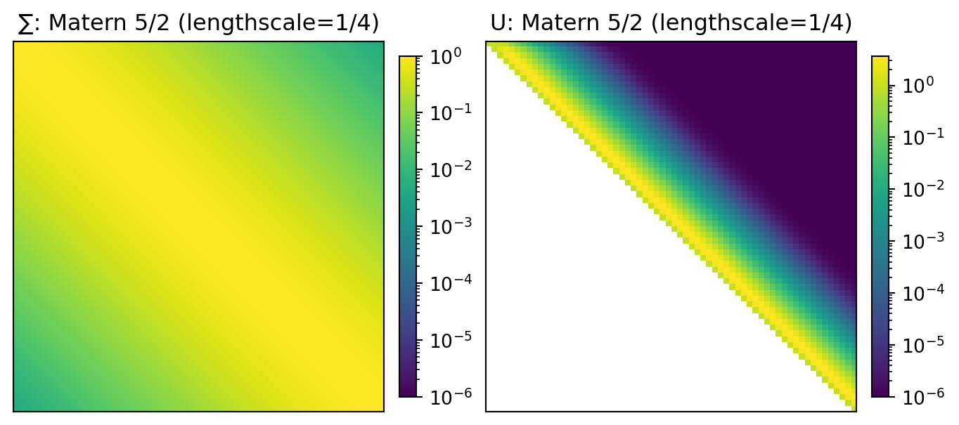
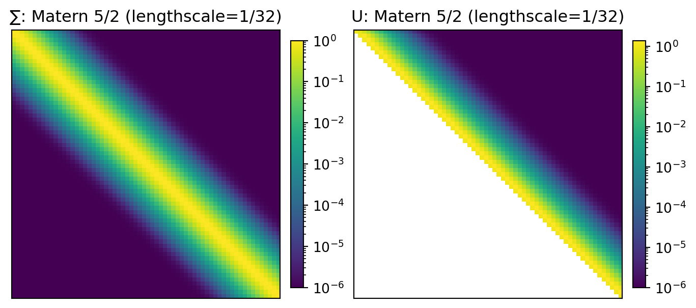
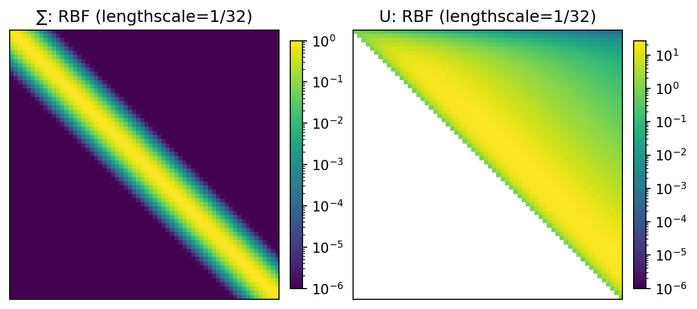
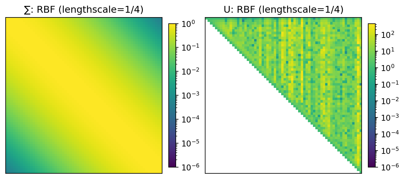
Figure 1 shows a selection of covariance matrices \Sigma and corresponding upper triangular factorizations U. Figure 1 (a) is the ideal case where a non-sparse \Sigma yields a highly sparse U,⁶ with just the diagonal and the adjacent entries being non-zero. This sparsity is an exceptional property of the exponential kernel, and Figure 1 (b) shows that changing to the Matérn 5/2 kernel yields a much less sparse U (but one that is still sparser than the covariance matrix itself). Figure 1 (c) drops the lengthscale from 1/4 to 1/32, which makes the covariance matrix much sparser (close to identity) while visually not changing U very much. Figure 1 (d) changes the kernel from Matérn 5/2, to RBF, making \Sigma look similar to before while U is essentially dense. However, the highest magnitude entries are still concentrated near the diagonal. Finally, Figure 1 (e) increases the lengthscale from 1/32 to 1/4, leading to a covariance matrix \Sigma that looks roughly similar to that of Figure 1 (b) but with a highly non-sparse U with many extreme entries (notice the colorbar range goes up to 10^3, compared with 10^1 or 10^0 for the other figures).

# Plot only these four kernels (as Quarto subfigures).
plot_keys = [(0.5, 4), (2.5, 4), (2.5, 32), (math.inf, 32), (math.inf, 4)]
for key in plot_keys:

    fig, axes = plt.subplots(
        1,
        2,
        constrained_layout=True,
        gridspec_kw={"width_ratios": [1, 1]},
    )

    U_abs = np.ma.array(np.abs(results[key]["U"]), mask=np.isnan(results[key]["U"]))
    cmap_U = plt.cm.viridis.copy()
    cmap_U.set_bad(color="white", alpha=0.0)

    eps = 1e-6
    cov_plot = np.abs(results[key]["cov"]) + eps
    U_plot = U_abs + eps

    im0 = axes[0].imshow(
        cov_plot,
        cmap="viridis",
        origin="upper",
        norm=LogNorm(vmin=eps, vmax=float(np.max(cov_plot))),
    )
    im1 = axes[1].imshow(
        U_plot,
        cmap=cmap_U,
        origin="upper",
        norm=LogNorm(vmin=eps, vmax=float(np.max(U_plot))),
    )

    axes[0].set_title(f"∑: {results[key]['name']}")
    axes[1].set_title(f"U: {results[key]['name']}")

    # Make the axes square and use log-scale colorbar ticks
    for ax in axes:
        ax.set_box_aspect(1)
        ax.set_xticks([])
        ax.set_yticks([])
    cb0 = fig.colorbar(im0, ax=axes[0], fraction=0.046, pad=0.04)
    cb1 = fig.colorbar(im1, ax=axes[1], fraction=0.046, pad=0.04)
    for cb in (cb0, cb1):
        cb.locator = LogLocator(base=10, subs=(1.0,))
        cb.formatter = LogFormatterMathtext(base=10)
        cb.update_ticks()

    plt.show()

(a) Exponential (lengthscale = 1/4)

(b) Matern 5/2 (lengthscale = 1/4)

(c) Matern 5/2 (lengthscale = 1/32)

(d) RBF (lengthscale = 1/32)

(e) RBF (lengthscale = 1/4)

Figure 1: Exact ∑, U for a selection of kernels on an evenly spaced grid in [0, 1].

Note 2: More about these particular kernels

These kernels are all members of the Matérn family of kernels with different values of \nu (which controls their smoothness). See Wikipedia for details.

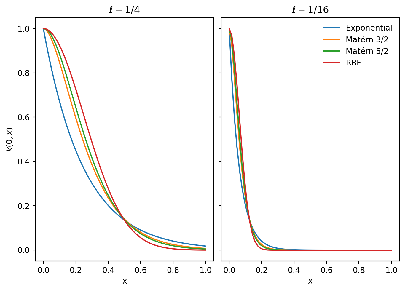
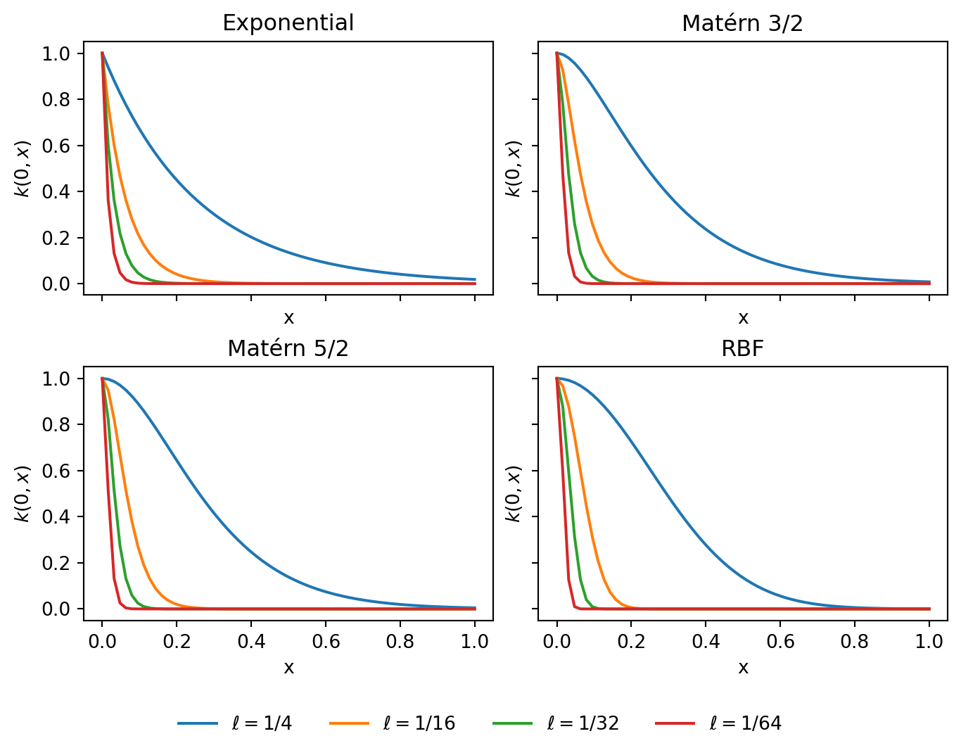
They are all stationary kernels with a lengthscale parameter \ell, which means k(x, x') depends only on the normalized distance \|x - x'\| / \ell. As such, it suffices to plot k(0, x). Figure 2 does this. The important takeaways are:

1. Among exponential \rightarrow Matern 3/2 \rightarrow Matern 5/2 \rightarrow RBF, the function’s initial decay gets slower, but its tail gets smaller. We get more short-range dependence and less long-range dependence.
2. For all these kernels, decreasing lengthscale causes faster decay.

There is a lot of theory behind these stationary kernels, and looking into this was a big rabbit hole I went into while writing this. Overall, my conclusion is not to overanalyze these differences. Stationary kernels on uniform 1D grids have a lot of idiosyncratic behaviour that might not be present on real data (the most interesting one was large entries with alternating signs in U). If you want to explore this, feel free to download this notebook and play around with the code, but I think it’s too much of a tangent to put in this post.

kernel_types = [
    (0.5, "Exponential"),
    (1.5, "Matérn 3/2"),
    (2.5, "Matérn 5/2"),
    (math.inf, "RBF"),
]
inv_lengthscales = sorted({inv for (_nu, inv) in results.keys()})


def cov0(nu: float, inv_lengthscale: int) -> np.ndarray:
    cov = results[(nu, inv_lengthscale)]["cov"]
    return cov[0, :]


# Plot 1: compare kernel types at two lengthscales (side-by-side)
inv_lengthscales_plot1 = [4, 16]
fig1, axes1 = plt.subplots(1, 2, sharey=True, constrained_layout=True)
for ax, inv_ls in zip(axes1, inv_lengthscales_plot1):
    for nu, label in kernel_types:
        ax.plot(x.flatten(), cov0(nu, inv_ls), label=label)
    ax.set_title(rf"$\ell = 1/{inv_ls}$")
    ax.set_xlabel("x")
axes1[0].set_ylabel(r"$k(0, x)$")
axes1[-1].legend(loc="best", frameon=False)
plt.show()


# Plot 2: for each kernel type, compare all lengthscales (2x2 grid)
cycle_colors = plt.rcParams["axes.prop_cycle"].by_key().get("color", [])
if not cycle_colors:
    cycle_colors = list(plt.cm.tab10.colors)
colors = {inv: cycle_colors[i % len(cycle_colors)] for i, inv in enumerate(inv_lengthscales)}

fig2, axes2 = plt.subplots(2, 2, sharex=True, sharey=True, constrained_layout=True)
axes2 = axes2.ravel()

legend_handles = []
legend_labels = [rf"$\ell = 1/{inv}$" for inv in inv_lengthscales]

for ax, (nu, label) in zip(axes2, kernel_types):
    for inv_ls in inv_lengthscales:
        (line,) = ax.plot(x.flatten(), cov0(nu, inv_ls), color=colors[inv_ls], label=rf"$\ell = 1/{inv_ls}$")
        if label == kernel_types[0][1]:
            legend_handles.append(line)
    ax.set_title(label)
    ax.set_ylabel(r"$k(0, x)$")
    ax.set_xlabel("x")

# Ensure the legend doesn't overlap with the plots
fig2.legend(legend_handles, legend_labels, loc="lower center", ncol=len(inv_lengthscales), frameon=False, bbox_to_anchor=(0.5, -0.1))
plt.show()

(a) Comparing kernel types with constant lengthscale

(b) Comparing lengthscales within each kernel type

Figure 2: Plots of kernel functions.

To understand the sparsity quantitatively, Table 1 shows the sparsity of U and \Sigma for each kernel and lengthscale (more than what was shown in Figure 1). Here an entry is considered zero if its absolute value is less than 10^{-4}.⁷

Average sparsity: The exponential kernel has a sparse U for all lengthscales (the constant sparsity is an artifact of the size of the matrix being 64\times64). The Matérn 3/2 and 5/2 kernels show a large amount of sparsity in U and \Sigma, decreasing as the lengthscale increases. The RBF kernel shows almost no sparsity in U, except for the smallest lengthscales.

Column-wise nnz: Clearly there is sparsity, but how uniform is it? For each column we calculate the number of non-zero (nnz) entries, using the same 10^{-4} criterion, then look at the quartiles across all columns. We count per column rather than per row because column i of U holds the coefficient vector \mathbf{c}_i (recall U = (I-L)^T, so rows of L become columns of U), which is exactly the quantity the Vecchia approximation will truncate later on. Except for the RBF kernels with larger lengthscales, we see that the nnz values are extremely uniform between columns.

Diagonal D: The final column also shows the minimum value of D. Low values can cause numerical stability issues. Because this is a bit of a tangential point, I’ve put further discussion in Note 3.

Summary: Overall, this suggests that U can not only be approximated reasonably well with a sparse matrix, but one with a fixed number of entries per column. As we will see later on, this forms the basis for the Vecchia approximation.

rows: list[dict[str, object]] = []
for (nu, inv_lengthscale), r in results.items():
    kernel_family = {
        0.5: "Exponential",
        1.5: "Matern 3/2",
        2.5: "Matern 5/2",
        math.inf: "RBF",
    }[nu]
    rows.append(
        {
            "inv_lengthscale": int(inv_lengthscale),
            "lengthscale": f"1/{int(inv_lengthscale)}",
            "kernel": kernel_family,
            "∑ avg sparsity": r["cov_avg_sparsity"],
            "U avg sparsity": r["U_avg_sparsity"],
            "U col nnz Q1": r["U_col_nnz_q1"],
            "U col nnz Q2": r["U_col_nnz_q2"],
            "U col nnz Q3": r["U_col_nnz_q3"],
            "min(D)": r["min_D"],
        }
    )

kernel_order = ["Exponential", "Matern 3/2", "Matern 5/2", "RBF"]
df = pd.DataFrame(rows)
df["kernel"] = pd.Categorical(df["kernel"], categories=kernel_order, ordered=True)
df = df.sort_values(["kernel", "inv_lengthscale"], ascending=[True, False]).reset_index(drop=True)

worst_idx = int(df["min(D)"].astype(float).idxmin())
worst = df.loc[worst_idx]

df = df.drop(columns=["inv_lengthscale"]).set_index(["kernel", "lengthscale"])

df.style.format(
    {
        "∑ avg sparsity": "{:.1%}",
        "U avg sparsity": "{:.1%}",
        "U col nnz Q1": "{:.0f}",
        "U col nnz Q2": "{:.0f}",
        "U col nnz Q3": "{:.0f}",
        "min(D)": "{:.2e}",
    }
)

Table 1: Near-sparsity (fraction of entries with abs(x) < 1e-4), column-wise nnz quartiles for U (count of entries with abs(x) ≥ 1e-4), and stability (min(D)) for all kernels considered.

		∑ avg sparsity	U avg sparsity	U col nnz Q1	U col nnz Q2	U col nnz Q3	min(D)
kernel	lengthscale
Exponential	1/64	72.5%	93.9%	2	2	2	8.69e-01
	1/32	50.5%	93.9%	2	2	2	6.38e-01
	1/16	18.5%	93.9%	2	2	2	3.98e-01
	1/4	0.0%	93.9%	2	2	2	1.19e-01
Matern 3/2	1/64	80.7%	79.5%	7	7	7	7.63e-01
	1/32	62.3%	76.7%	8	8	8	3.44e-01
	1/16	34.3%	74.0%	9	9	9	9.16e-02
	1/4	0.0%	71.4%	10	10	10	2.66e-03
Matern 5/2	1/64	83.5%	74.0%	9	9	9	7.09e-01
	1/32	67.3%	66.2%	12	12	12	2.22e-01
	1/16	40.0%	61.3%	14	14	14	2.85e-02
	1/4	0.0%	58.9%	15	15	15	9.08e-05
RBF	1/64	86.4%	47.8%	17	20	20	5.23e-01
	1/32	75.2%	0.0%	17	33	48	8.49e-03
	1/16	55.1%	0.0%	17	33	48	-9.22e-08
	1/4	0.0%	0.0%	17	33	48	-5.68e-13

Note 3: More on min(D)

Remember that the matrix factor is not U, it is UD^{-1/2}, effectively scaling the columns of U by \frac{1}{\sqrt{D_{ii}}}. Very small entries in D will cause this scaling to be large and amplifies rounding error. Intuitively, small D_{ii} means that point i is almost deterministically explained by its neighbours, and also implies that the covariance matrix is nearly singular.

\min(D) is smallest for the RBF kernels with large lengthscales. The last rows of Table 1 show negative numbers, which is a sign of numerical error (it should never be negative). In such situations, the Vecchia approximation may not work very well.

2.3 Ordering: the scourge of Vecchia

After reading Section 2.2 you may be feeling some cautious optimism: even if U isn’t always sparse, there genuinely are cases where it is very uniformly and predictably sparse. Unfortunately, this is an instance where toy examples on [0, 1] can be misleading. The factorization from Section 2.1 is highly dependent on the ordering of points, and it turns out that feeding the points in increasing order is a nearly best-case scenario. In practice, ordering will be a persistent problem throughout the Vecchia approximation that will either increase cost, reduce accuracy, or require special treatment.

2.3.1 Why does ordering matter?

The order of points doesn’t normally matter for exact GPs. For GP priors, a permutation \pi of the inputs just creates a new covariance matrix \tilde\Sigma where \tilde\Sigma_{ij} = \Sigma_{\pi(i), \pi(j)} (essentially permuting the rows and columns of \Sigma), which just permutes the rows of the variable \mathbf{y}.

This carries through to the factorization. If we permute the rows and columns of UD^{-1/2} by \pi, it will still be a valid factorization of \tilde\Sigma^{-1}. However, after this permutation this matrix will (in general) no longer be upper triangular. A new upper triangular factorization of \tilde\Sigma^{-1} will need to be computed, and its structure and elements may look very different from the original U and D.

2.3.2 Looking empirically

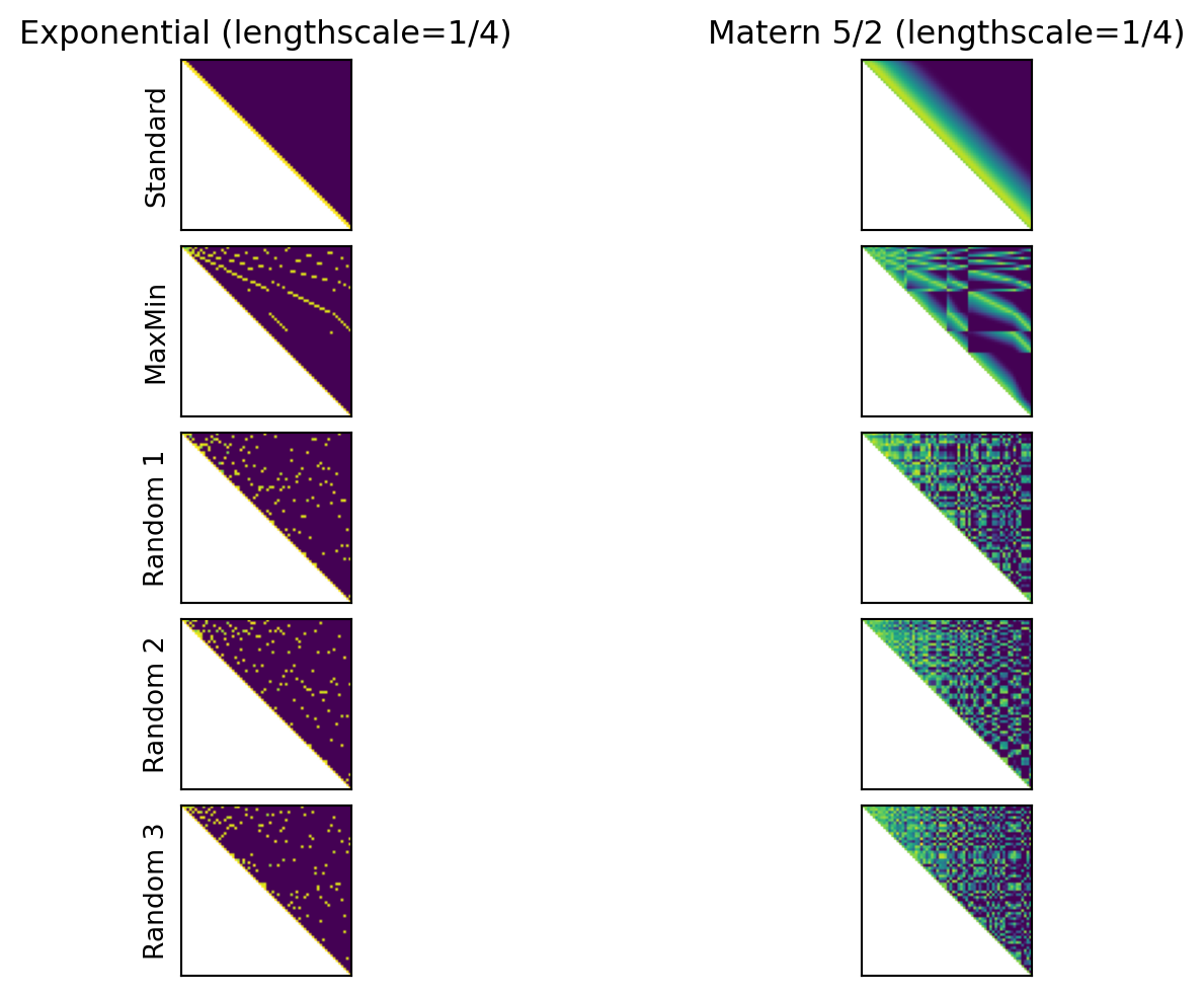
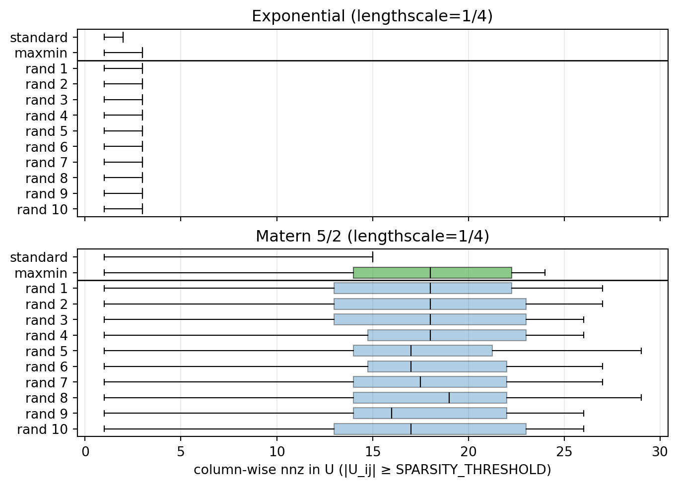
We will use the same exponential and Matérn 5/2 kernels with \ell = 1/4 (from Figure 1 (a) and Figure 1 (b)), and look at how the factorization changes with different orderings of the points. Figure 3 (a) compares U with the standard ordering (increasing x), maxmin ordering (choosing points greedily sequentially by maximum distance to already chosen points), and 3 random orderings. While the standard ordering yields a clean diagonal, the random ordering has non-zero entries all over the place (although that is hardly surprising since the ordering is random), and maxmin has an interesting banded structure. Figure 3 (b) shows the column-wise non-zero count. The exponential kernel is barely affected by the ordering: its Markov property means each point is screened by its nearest preceding point on each side, so every ordering yields at most 3 non-zero entries per column. The Matérn 5/2 kernel reveals the real problem: while the standard ordering has a constant number of non-zero entries per column (except for the first few columns, which run out of preceding points), both maxmin and the random orderings have a much wider range of values, with an interquartile range of ~10 and maximum column counts of ~25 or more (compared to a constant 15 for the standard ordering).

This will leave several bad options for Vecchia sparse approximations:

1. Vary the enforced sparsity per column (in principle not an issue, but in practice determining how many nnz values to include will incur some overhead).
2. Enforce very little sparsity. This could approximate every column well, but the approximation would be nearly dense.
3. Enforce a high level of sparsity and accept losing accuracy on some columns.

x = np.linspace(0, 1, 64).reshape(-1, 1)
x_permuted = [rng.permutation(x) for _ in range(10)]

# Create a greedy maxmin ordering of the set (a permutation of x)
x_flat = x[:, 0]
n = x_flat.shape[0]
chosen = np.zeros(n, dtype=bool)
order: list[int] = []

# Since x is sorted, the endpoints are indices 0 and n-1.
order.extend([0, n - 1])
chosen[0] = True
chosen[n - 1] = True

min_dist = np.minimum(np.abs(x_flat - x_flat[0]), np.abs(x_flat - x_flat[n - 1]))
min_dist[chosen] = -np.inf

for _ in range(n - 2):
    idx = int(np.argmax(min_dist))
    order.append(idx)
    chosen[idx] = True
    min_dist = np.minimum(min_dist, np.abs(x_flat - x_flat[idx]))
    min_dist[chosen] = -np.inf

x_maxmin = x[np.array(order)]
assert x_maxmin.shape == x.shape
assert np.allclose(np.sort(x_maxmin[:, 0]), np.sort(x[:, 0]))

# Compute U and column-wise nnz under different orderings
nus = [0.5, 2.5]
kernel_names: dict[float, str] = {}
U_for_plot: dict[float, list[np.ndarray]] = {}
U_col_nnz: dict[float, list[np.ndarray]] = {}

for nu in nus:
    kernel, name = params_to_kernel[(nu, 4)]
    kernel_names[nu] = name

    U_for_plot[nu] = []
    U_col_nnz[nu] = []

    # Standard ordering
    cov = kernel(x, x)
    U, _D = get_U_and_D_exact(cov)
    U_for_plot[nu].append(U)
    U_col_nnz[nu].append(num_nnz_per_col(U))

    # Maxmin ordering
    cov_maxmin = kernel(x_maxmin, x_maxmin)
    U_maxmin, _D_maxmin = get_U_and_D_exact(cov_maxmin)
    U_for_plot[nu].append(U_maxmin)
    U_col_nnz[nu].append(num_nnz_per_col(U_maxmin))

    # Random orderings
    for j, x_perm in enumerate(x_permuted):
        cov_perm = kernel(x_perm, x_perm)
        U_perm, _D_perm = get_U_and_D_exact(cov_perm)
        if j < 3:
            U_for_plot[nu].append(U_perm)
        U_col_nnz[nu].append(num_nnz_per_col(U_perm))


# Plot 1 (subfigure a): pictures of U, transposed to be tall
order_titles = ["Standard", "MaxMin", "Random 1", "Random 2", "Random 3"]

cmap_U = plt.cm.viridis.copy()
cmap_U.set_bad(color="white", alpha=0.0)

eps = 1e-6

fig1, axes1 = plt.subplots(5, 2, constrained_layout=True, sharex=True, sharey=True)

for kcol, nu in enumerate(nus):
    vmax = float(
        np.max(
            [
                np.max(np.abs(Ui[~np.isnan(Ui)])) if np.any(~np.isnan(Ui)) else 0.0
                for Ui in U_for_plot[nu]
            ]
        )
        + eps
    )
    norm = LogNorm(vmin=eps, vmax=vmax)

    for r, title in enumerate(order_titles):
        ax = axes1[r, kcol]

        U_here = U_for_plot[nu][r]
        U_abs = np.ma.array(np.abs(U_here), mask=np.isnan(U_here))
        U_plot = U_abs + eps

        ax.imshow(U_plot, cmap=cmap_U, origin="upper", norm=norm)
        ax.set_box_aspect(1)
        ax.set_xticks([])
        ax.set_yticks([])

        if r == 0:
            ax.set_title(kernel_names[nu])
        if kcol == 0:
            ax.set_ylabel(title)

plt.show()
plt.close(fig1)


# Plot 2 (subfigure b): box plot of column-wise nnz, transposed to be tall
labels = ["standard", "maxmin"] + [f"rand {i + 1}" for i in range(len(x_permuted))]
positions = np.arange(len(labels), 0, -1)  # top = standard

fig2, axes2 = plt.subplots(2, 1, constrained_layout=True, sharex=True)
for ax, nu in zip(axes2, nus):
    data = U_col_nnz[nu]  # [standard] + 10 random
    # Set whis=[0, 100] to extend whiskers to min/max (and showfliers=False to hide outliers)
    bp = ax.boxplot(
        data,
        vert=False,
        positions=positions,
        widths=0.7,
        patch_artist=True,
        showfliers=False,
        whis=[0, 100],  # whiskers show min and max
    )

    # Clear delineation between the deterministic orderings (standard/maxmin) and random orderings.
    ax.axhline(y=positions[1] - 0.5, color="black", linewidth=1.0)

    for i, box in enumerate(bp["boxes"]):
        if i == 0:
            box.set_facecolor("tab:orange")
            box.set_alpha(0.65)
        elif i == 1:
            box.set_facecolor("tab:green")
            box.set_alpha(0.55)
        else:
            box.set_facecolor("tab:blue")
            box.set_alpha(0.35)
        box.set_edgecolor("black")
        box.set_linewidth(0.8)

    for key in ("whiskers", "caps", "medians"):
        for artist in bp[key]:
            artist.set_color("black")
            artist.set_linewidth(0.8)

    ax.set_yticks(positions)
    ax.set_yticklabels(labels)
    ax.set_title(kernel_names[nu])
    ax.grid(axis="x", alpha=0.25)

axes2[-1].set_xlabel(r"column-wise nnz in U (|U_ij| ≥ SPARSITY_THRESHOLD)")

plt.show()
plt.close(fig2)

(a) U under standard, maxmin, and random orderings.

(b) Column-wise non-zeros in U under standard, maxmin, and random orderings. Whiskers show min and max.

Figure 3: Effect of ordering on the upper-triangular factor U (subfigure a) and column-wise non-zeros (subfigure b).

2.3.3 Where does the non-uniformity come from?

Recall \mathbf{c}_i (Equation 2), which controls the off-diagonal entries in U. It will be large whenever the covariance between i and any of the preceding points is large. Roughly, each large non-zero covariance should produce a large off-diagonal entry. In the standard ordering, every point sees the points to its left, which will contain the same amount of “relevant” points. In non-standard orderings, points will see a mixture of points to their left and right. In some cases, a point may not have many close points to its left and right yet (e.g. if 0.5 is the first point, it sees nothing). In other cases, a point may have many close points (e.g. if 0.49 is the last point placed, it will see \{\ldots, 0.47, 0.48, \mathbf{*}, 0.5, 0.51, \ldots\}).

2.3.4 Conclusion for ordering

As much as I would like to say “… and here is how you get the optimal ordering”, as far as I can tell this is an unsolved problem (or at least expensive enough to solve that it would defeat the point of using the Vecchia approximation in the first place).

This is just a general downside to Vecchia: order will matter, you won’t know how to set it, and it will negatively impact the approximation quality.

2.4 Summary of Section 2

Key points:

• Factorization:
  • We created a factorization \Sigma^{-1} = U D^{-1} U^T, where U is upper triangular and D is diagonal.
  • U=(I-L)^T where L is lower triangular
  • The entries of L (Equation 3) come from a vector \mathbf{c} (Equation 2), which comes from the standard GP posterior equations, which you would use if sampling sequentially.
• Sparsity: in some toy examples we found that U is often sparse (Section 2.2), although its sparsity structure depends on the covariance matrix and the ordering of the inputs (Section 2.3).

3 Vecchia approximation for multivariate Gaussian distributions

3.1 The core of the approximation

At its core, the Vecchia approximation is just to replace the index set “:i” (shorthand for 1, \ldots, (i-1)) with a smaller index set N(i) \subseteq \{1, \ldots, i-1\} of length at most m (which is called the neighbourhood of i). Otherwise, everything else is the same as Section 2.1:

• We will construct a vector

  \tilde{\mathbf{c}}_i = \Sigma_{N(i), N(i)}^{-1} \Sigma_{N(i), i} \tag{5}

  analogous to Equation 2.

• We will construct a lower triangular matrix \tilde L with the same structure as L (Equation 3), but using \tilde{\mathbf{c}} vectors instead of \mathbf{c} vectors (more detail on this below), then set \tilde U = (I - \tilde L)^T.

• We will construct the diagonal matrix \tilde D analogously to D, modifying Equation 1 to get

  \tilde\sigma^2_i = \Sigma_{i,i} - \underbrace{\Sigma_{i, N(i)} \Sigma_{N(i), N(i)}^{-1}}_{\tilde{\mathbf{c}}_i^T} \Sigma_{N(i), i} \tag{6}

  then set

  \tilde D = \mathrm{diag}(\tilde\sigma^2_1, \ldots, \tilde\sigma^2_n) \ . \tag{7}

• Our total factorization is then \tilde\Sigma^{-1} = \tilde U \tilde D^{-1} \tilde U^T. Of course, we don’t usually form \tilde\Sigma^{-1} explicitly (that would defeat the point of the approximation in most settings), but instead use \tilde U and \tilde D directly in downstream GP operations, exactly as described in Note 1.

Hopefully this makes sense at a high level. Now let’s clarify the construction of \tilde L, which was described imprecisely above. Recall the exact structure of L from Equation 3:

L = \begin{pmatrix} 0 & 0 & 0 & \cdots & 0 \\ c_{2,1} & 0 & 0 & \cdots & 0 \\ c_{3,1} & c_{3,2} & 0 & \cdots & 0 \\ \vdots & \vdots & \vdots & \ddots & \vdots \\ c_{n,1} & c_{n,2} & c_{n,3} & \cdots & 0 \end{pmatrix} \ .

The ith row of L needs (i-1) off diagonal entries, but the vector \tilde{\mathbf{c}}_i has at most m entries: a shape mismatch! Instead, we interpret \tilde{\mathbf{c}}_i as parameterizing only the non-zero entries of the ith row of L. Specifically, we have

\tilde L_{i,j} = \begin{cases} 0 & \text{if } j \geq i \text{ (only lower triangular part can be non-zero)} \\ \tilde{c}_{i,k} & \text{if } j = N(i)[k] \text{ for some } k \in \{1, \ldots, m\} \\ 0 & \text{otherwise (}j\text{ is not in the neighbourhood of }i\text{)} \end{cases} \ . \tag{8}

This structure guarantees that the ith row of \tilde L will have exactly \left| N(i) \right| \leq m non-zero entries, implying that columns of U will have \leq m non-zero off-diagonal entries.

Parameters: the only “parameters” that control the approximation are the neighbourhood sets N(i): no tolerances, bandwidths, inducing points, etc. Even m is just a quantity derived from the neighbourhood sets (m=\max_i |N(i)|).

3.2 Speed and memory analysis for constructing the approximation

Let’s put aside the construction of the neighbourhoods N(1), \ldots, N(n) for now and assume |N(i)| = m for all i. The Vecchia approximation requires:

Step	Memory cost	Time cost
Constructing \Sigma_{N(i), i} (size at most m \times 1) for each i.	O(m) (we don’t need to store these, so only 1 m-vector is needed)	O(nm)
Constructing \tilde{\mathbf{c}}_i = \Sigma_{N(i), N(i)}^{-1} \Sigma_{N(i), i} for each i.	O(m^2) to construct the matrix \Sigma_{N(i), N(i)} once, O(nm) to store all vectors.	O(nm^3) (time taken to solve n linear systems of size m\times m)
Constructing \tilde U from \tilde{\mathbf{c}} vectors	O(nm)	O(nm)
Constructing \tilde D by sequentially constructing the diagonal entries \tilde\sigma^2_i	O(n)	O(nm) (\Sigma_{i,i} is a constant-time operation, and \tilde{\mathbf{c}}_i^T \Sigma_{N(i), i} is O(m) repeated n times)

Overall, this gives a time cost of O(nm^3) and a memory cost of O(nm). If m\ll n, this will be a significant speedup over the full covariance matrix. However, as m\to n, the cost will actually be higher than exact GP inference (tending to O(n^4) instead of O(n^3) for the exact Cholesky decomposition). So, the approximation really only makes sense for small m.

Reminder 1: this is the cost of constructing the approximation- using it has a different cost (see Note 1), generally O(nm).

Reminder 2: this cost excluded the cost of constructing the neighbourhood sets N(i).

3.3 Interpretation of the approximation

There are two broad interpretations of Vecchia. The first is that it is exact inference in an approximate model. In this interpretation, we are defining the sequential sampling procedure such that each variable is only conditionally dependent on the previous variables in N(i), instead of all previous variables like in the full GP. Note that because all conditional distributions are Gaussians, the full model is still a multivariate Gaussian (a GP), just a different one than the one we started with. In this “approximate model”, the sparse factorization is exact. This seems to be how most papers present Vecchia: essentially a special model designed for fast inference.

This is not my preferred interpretation, mostly because in my area of work it makes sense to use whatever approximation is most appropriate, and in different settings this could be low-rank approximations, variational approximations, etc. The commonality between all these approximations is the underlying GP model, so I’d rather think of Vecchia as approximate inference in the exact GP model. In this interpretation, we are pre-committing to a level of sparsity in the factorization, pre-committing to which specific entries will be non-zero, and then filling these entries “optimally” with the exact GP posterior equations.⁸

3.4 Experimental investigation

Now let’s see how the Vecchia approximation looks in practice for a variety of neighbourhood sets.

def get_U_and_D_vecchia(Sigma, neighbourhood_sets: dict[int, list[int]]) -> tuple[np.ndarray, np.ndarray]:

    # Validate neighbourhood sets
    for i in range(len(Sigma)):
        assert i in neighbourhood_sets, f"Point {i} does not have a neighbourhood set"
        for j in neighbourhood_sets[i]:
            assert j < i, "Neighbourhood set must contain only previous points"
   
    # Construct U and D like before
    U_T = np.eye(Sigma.shape[0])  # unit diagonal
    D = np.empty(Sigma.shape[0])

    D[0] = Sigma[0, 0]

    for i in range(1, Sigma.shape[0]):
        idx = neighbourhood_sets[i]
        if len(idx) == 0:
            D[i] = Sigma[i, i]
            continue

        # Use np.ix_ to extract the submatrix (avoids advanced-indexing diagonal behavior).
        Sigma_prev = Sigma[np.ix_(idx, idx)]
        Sigma_slice = Sigma[i, idx]
        c_i = np.linalg.solve(Sigma_prev, Sigma_slice)
        U_T[i, idx] = -c_i
        D[i] = Sigma[i, i] - np.dot(c_i, Sigma_slice)

    U = U_T.T.copy()
    U[np.tril_indices(Sigma.shape[0], k=-1)] = np.nan
    return U, D

3.4.1 Varying the number of neighbours

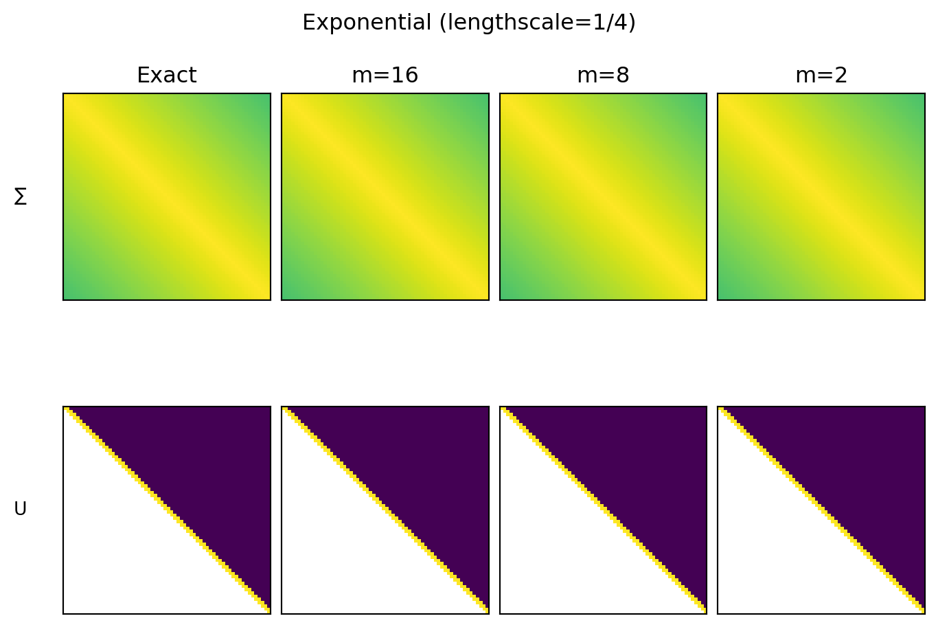
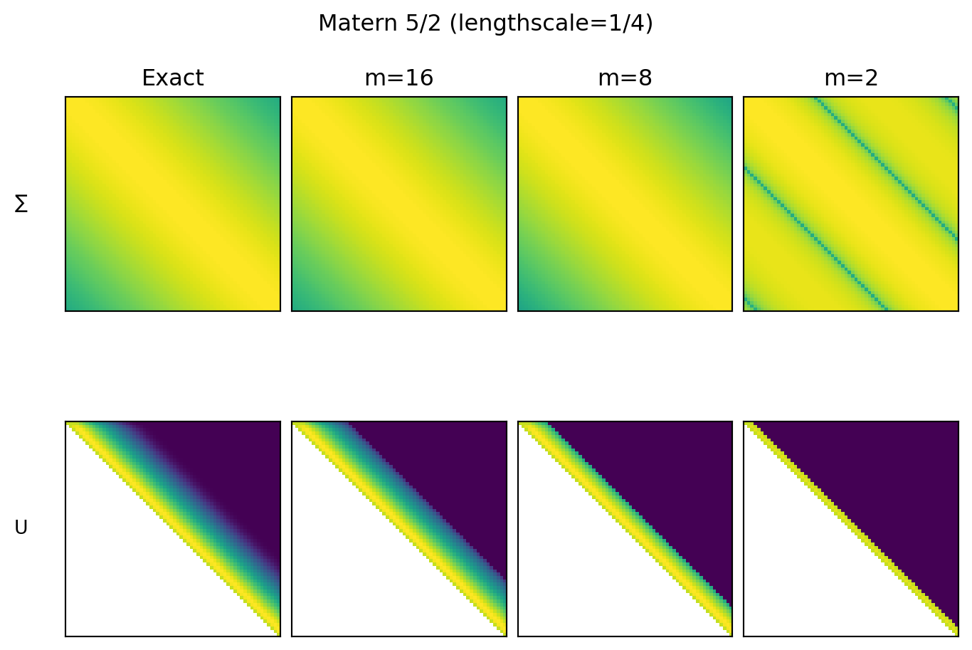
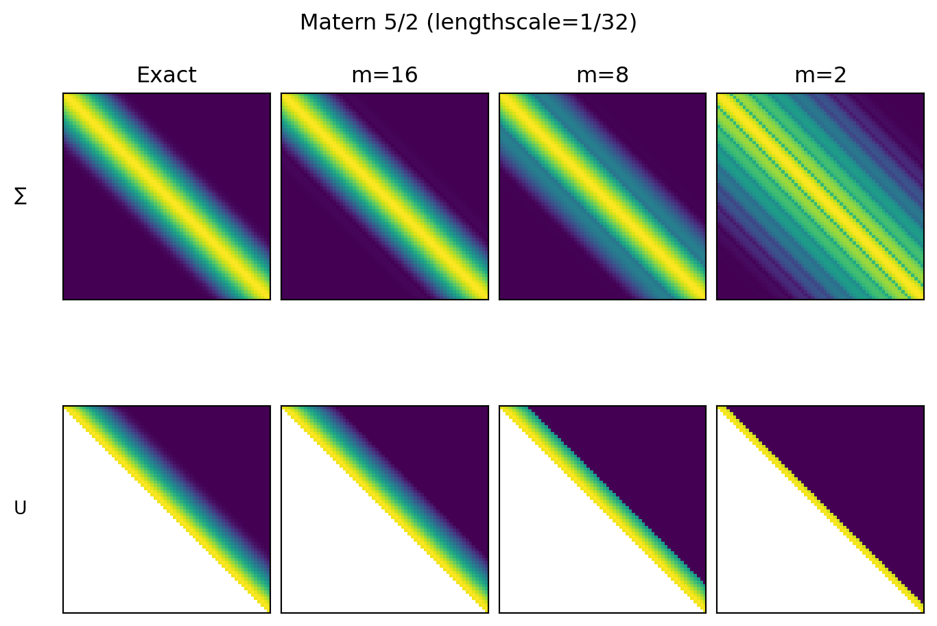
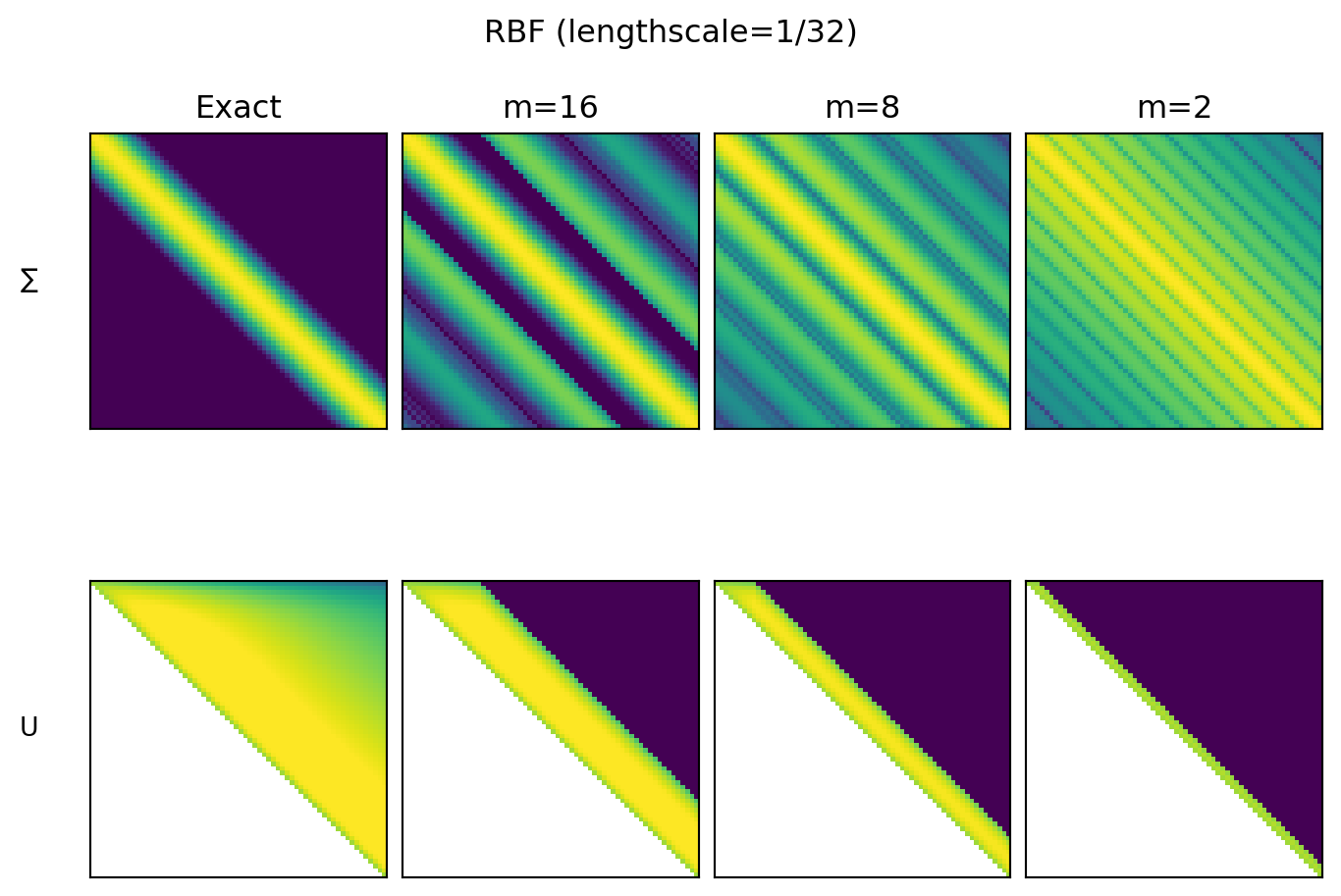
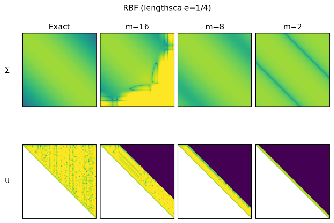
Let’s re-visit the 5 covariance matrices from Figure 1, which we examined in detail earlier. When the matrices U were sparse, the sparsity was concentrated around the neighbouring points (hence the diagonal bands). We will now apply Vecchia to these matrices using the nearest m points as the neighbourhood sets.

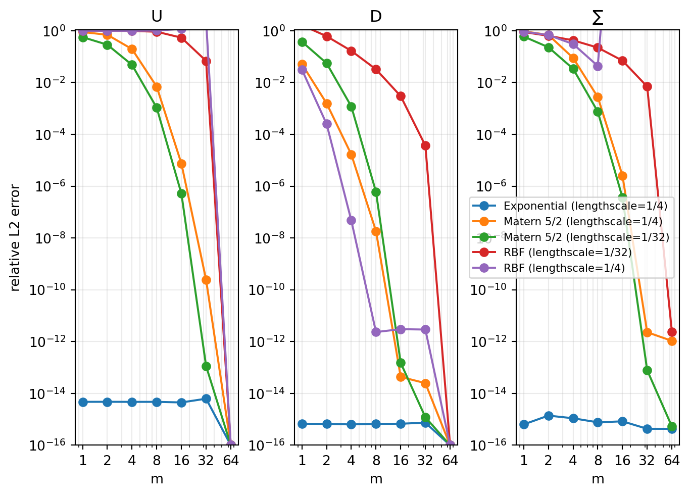
Figure 4 shows the results. For the exponential and Matern 5/2 kernels the approximation looks pretty good, except for m=2 with Matern 5/2, where spurious “bands” are introduced.⁹ For the RBF kernel, the approximation looks surprisingly poor, even at m=16. Figure 5 shows the relative L2 errors in the reconstruction of U, D, and \Sigma, showing clear improvement as m increases (except for sometimes numerical error when calculating \Sigma).

#
# This section reuses `results` (exact cov/U/D for many kernels)
# and `get_U_and_D_vecchia` (Vecchia factor construction) defined above.

m_values = [1, 2, 4, 8, 16, 32, 64]


def previous_m_neighbourhood_sets(n: int, m: int) -> dict[int, list[int]]:
    # N(i) = {max(0, i-m), ..., i-1}
    return {i: list(range(max(0, i - m), i)) for i in range(n)}


def reconstruct_Sigma_from_U_D(U: np.ndarray, D: np.ndarray) -> np.ndarray:
    # From Σ^{-1} = U D^{-1} U^T, we have Σ = U^{-T} diag(D) U^{-1}.
    # (Equivalently: X = U^{-T} D^{1/2}; Σ = X X^T.)
    U0 = np.nan_to_num(U, nan=0.0)
    n = U0.shape[0]
    U_inv = np.linalg.solve(U0, np.eye(n))
    return U_inv.T @ np.diag(np.asarray(D)) @ U_inv


def rel_l2_error(A: np.ndarray, B: np.ndarray) -> float:
    A0 = np.nan_to_num(A, nan=0.0)
    B0 = np.nan_to_num(B, nan=0.0)
    denom = np.linalg.norm(A0)
    num = np.linalg.norm(A0 - B0)
    return float(num / denom) if denom > 0 else float(num)


# Compute Vecchia U/D and implied Σ + errors for every kernel and m.
vecchia: dict[tuple[float, int], dict[int, dict[str, object]]] = {key: {} for key in results}

for key, info in results.items():
    Sigma_exact = np.asarray(info["cov"])
    U_exact = np.asarray(info["U"])
    D_exact = np.asarray(info["D"])

    n = Sigma_exact.shape[0]
    assert Sigma_exact.shape == (n, n)
    assert U_exact.shape == (n, n)
    assert D_exact.shape == (n,)

    for m in m_values:
        neighbourhood_sets = previous_m_neighbourhood_sets(n, m)
        U_m, D_m = get_U_and_D_vecchia(Sigma_exact, neighbourhood_sets)
        Sigma_m = reconstruct_Sigma_from_U_D(U_m, D_m)

        vecchia[key][m] = {
            "U": U_m,
            "D": D_m,
            "cov": Sigma_m,
            "err_U": rel_l2_error(U_exact, U_m),
            "err_D": rel_l2_error(D_exact, D_m),
            "err_cov": rel_l2_error(Sigma_exact, Sigma_m),
        }


# Plot comparison grids for the same 5 kernels as Figure 1.
plot_keys = [(0.5, 4), (2.5, 4), (2.5, 32), (math.inf, 32), (math.inf, 4)]
show_ms = [None, 16, 8, 2]
col_titles = ["Exact", "m=16", "m=8", "m=2"]

cmap_U = plt.cm.viridis.copy()
cmap_U.set_bad(color="white", alpha=0.0)

eps = 1e-6

for key in plot_keys:
    name = str(results[key]["name"])

    Sigma_exact = np.asarray(results[key]["cov"])
    U_exact = np.asarray(results[key]["U"])

    Sigmas = [Sigma_exact] + [np.asarray(vecchia[key][m]["cov"]) for m in show_ms[1:]]
    Us = [U_exact] + [np.asarray(vecchia[key][m]["U"]) for m in show_ms[1:]]

    # Shared color scales per row (cov row, U row).
    vmax_cap = 1e1
    cov_vmax = float(max(np.max(np.abs(S) + eps) for S in Sigmas))
    U_vmax = float(
        max(
            (np.max(np.abs(U_here[~np.isnan(U_here)])) if np.any(~np.isnan(U_here)) else 0.0)
            for U_here in Us
        )
        + eps
    )
    cov_vmax = min(cov_vmax, vmax_cap)
    U_vmax = min(U_vmax, vmax_cap)
    cov_norm = LogNorm(vmin=eps, vmax=cov_vmax)
    U_norm = LogNorm(vmin=eps, vmax=U_vmax)

    fig, axes = plt.subplots(2, 4, constrained_layout=True)

    for c in range(4):
        cov_plot = np.abs(Sigmas[c]) + eps
        axes[0, c].imshow(cov_plot, cmap="viridis", origin="upper", norm=cov_norm)

        U_abs = np.ma.array(np.abs(Us[c]), mask=np.isnan(Us[c]))
        U_plot = U_abs + eps
        axes[1, c].imshow(U_plot, cmap=cmap_U, origin="upper", norm=U_norm)

        for r in (0, 1):
            axes[r, c].set_box_aspect(1)
            axes[r, c].set_xticks([])
            axes[r, c].set_yticks([])

        axes[0, c].set_title(col_titles[c])

    axes[0, 0].set_ylabel("∑", rotation=0, labelpad=20, ha="right", va="center")
    axes[1, 0].set_ylabel("U", rotation=0, labelpad=20, ha="right", va="center")
    fig.suptitle(name)

    plt.show()
    plt.close(fig)

(a) Exponential (lengthscale = 1/4)

(b) Matern 5/2 (lengthscale = 1/4)

(c) Matern 5/2 (lengthscale = 1/32)

(d) RBF (lengthscale = 1/32)

(e) RBF (lengthscale = 1/4)

Figure 4: Vecchia approximation of ∑ and U for different neighbourhood sizes m (previous-point neighbourhoods).

fig, axes = plt.subplots(1, 3, constrained_layout=True)

y_floor = 1e-16  # Avoid log(0) in plots.

for key in plot_keys:
    name = str(results[key]["name"])
    ms = np.array(m_values, dtype=float)

    err_U = np.array([float(vecchia[key][m]["err_U"]) for m in m_values], dtype=float)
    err_D = np.array([float(vecchia[key][m]["err_D"]) for m in m_values], dtype=float)
    err_cov = np.array([float(vecchia[key][m]["err_cov"]) for m in m_values], dtype=float)

    err_U = np.maximum(err_U, y_floor)
    err_D = np.maximum(err_D, y_floor)
    err_cov = np.maximum(err_cov, y_floor)

    axes[0].plot(ms, err_U, marker="o", linewidth=1.5, label=name)
    axes[1].plot(ms, err_D, marker="o", linewidth=1.5, label=name)
    axes[2].plot(ms, err_cov, marker="o", linewidth=1.5, label=name)

for ax, title in zip(axes, ["U", "D", "∑"]):
    ax.set_xscale("log")
    ax.set_yscale("log")
    ax.set_xticks(m_values)
    ax.set_xticklabels([str(m) for m in m_values])
    ax.grid(alpha=0.25, which="both")
    ax.set_title(title)
    ax.set_xlabel("m")
    ax.set_ylim(bottom=y_floor, top=1.1)

axes[0].set_ylabel("relative L2 error")
axes[2].legend(fontsize=8, loc="best")

plt.show()
plt.close(fig)

Figure 5: Relative L2 reconstruction error vs neighbourhood size m (log-x, log-y; y-axis capped at 1).

3.4.2 Varying the neighbourhood set

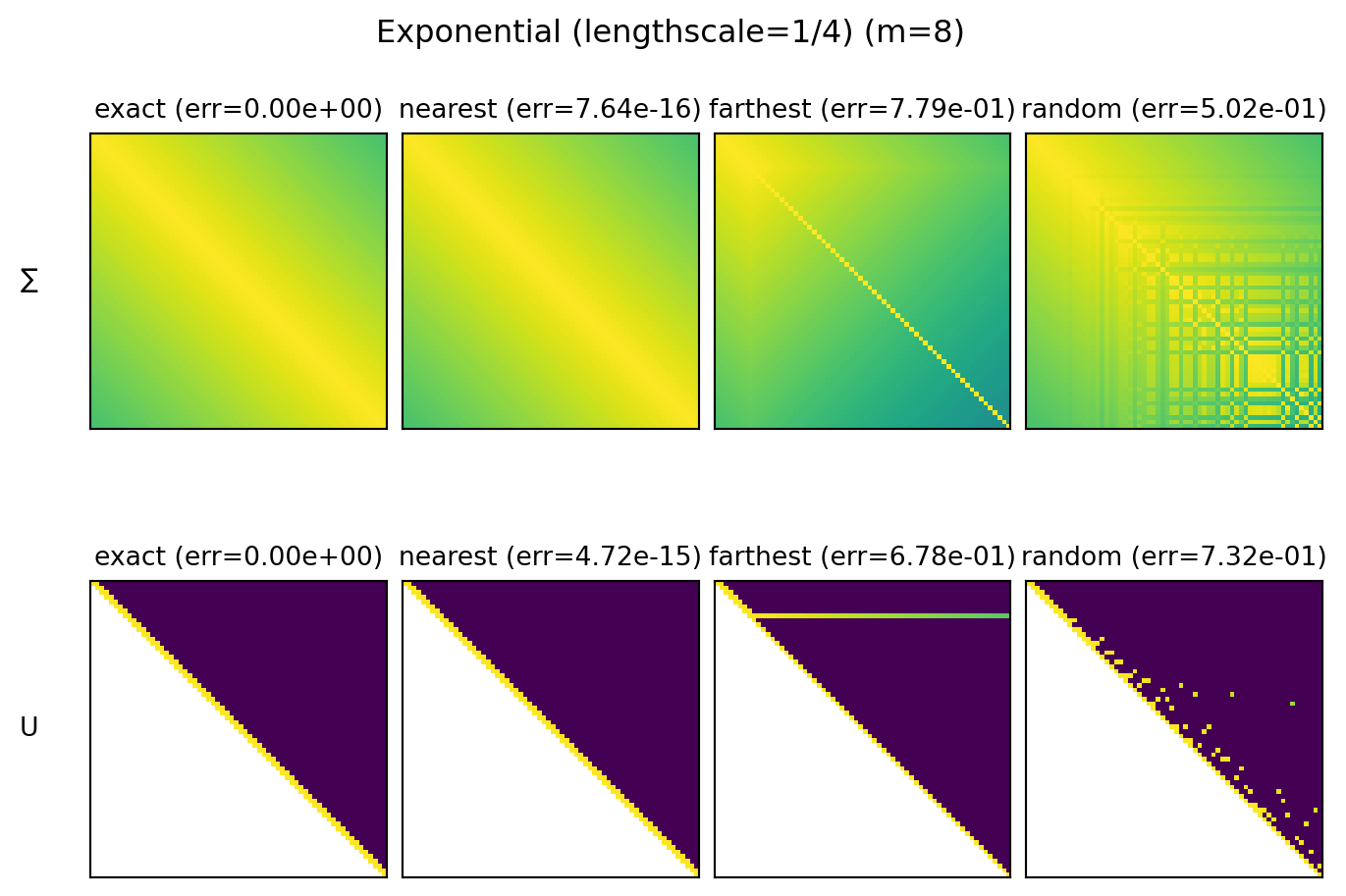
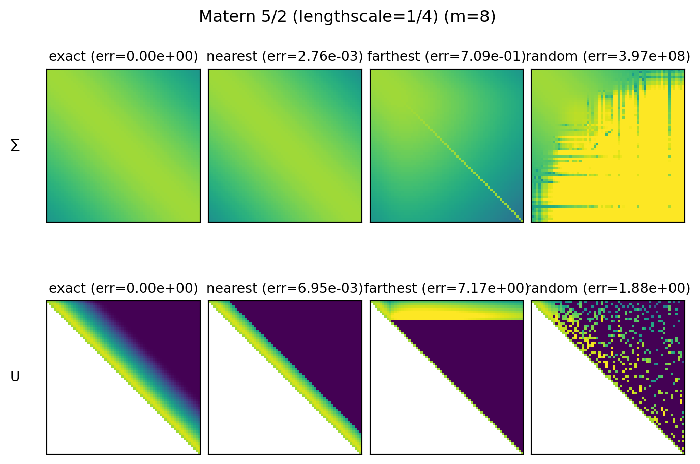
Figure 6 shows the result of changing the neighbourhood set from “nearest” to farthest points or a random set of points on the kernels from Figure 4 (a) and Figure 4 (b) (which both had good reconstruction errors for m=8). Farthest and random points are both significantly worse, which makes sense because the enforced sparsity structure looks nothing like the exact U matrix.

m = 8
kernel_keys = [(0.5, 4), (2.5, 4)]

# Recreate the 64-point grid (matches the earlier experiment).
x = np.linspace(0, 1, 64).reshape(-1, 1)

# Use a dedicated RNG so this figure stays stable even if earlier cells change.
rng_neighbourhood = np.random.default_rng(123)


def neighbourhood_sets_by_distance(
    x: np.ndarray, m: int, *, mode: str, rng: np.random.Generator
) -> dict[int, list[int]]:
    n = x.shape[0]
    x_flat = x[:, 0] if x.ndim == 2 else x

    neighbourhood_sets: dict[int, list[int]] = {0: []}
    for i in range(1, n):
        prev = np.arange(i)
        k = min(m, i)

        if k == i:
            idx = prev
        else:
            dists = np.abs(x_flat[i] - x_flat[prev])
            if mode == "nearest":
                idx = prev[np.argsort(dists)[:k]]
            elif mode == "farthest":
                idx = prev[np.argsort(dists)[-k:]]
            elif mode == "random":
                idx = rng.choice(prev, size=k, replace=False)
            else:
                raise ValueError(f"Unknown mode: {mode}")

        neighbourhood_sets[i] = np.sort(idx).tolist()

    return neighbourhood_sets


cmap_U = plt.cm.viridis.copy()
cmap_U.set_bad(color="white", alpha=0.0)

eps = 1e-6

# Fix the neighbourhood sets once (so "random" is a single ordering shared across kernels).
nh_by_mode = {
    mode: neighbourhood_sets_by_distance(x, m, mode=mode, rng=rng_neighbourhood)
    for mode in ["nearest", "farthest", "random"]
}

for key in kernel_keys:
    name = str(results[key]["name"])
    Sigma_exact = np.asarray(results[key]["cov"])
    U_exact = np.asarray(results[key]["U"])

    approx: dict[str, dict[str, object]] = {}
    for mode in ["nearest", "farthest", "random"]:
        nh = nh_by_mode[mode]
        U_m, D_m = get_U_and_D_vecchia(Sigma_exact, nh)
        Sigma_m = reconstruct_Sigma_from_U_D(U_m, D_m)

        approx[mode] = {
            "cov": Sigma_m,
            "U": U_m,
            "err_cov": rel_l2_error(Sigma_exact, Sigma_m),
            "err_U": rel_l2_error(U_exact, U_m),
        }

    Sigmas = [Sigma_exact, np.asarray(approx["nearest"]["cov"]), np.asarray(approx["farthest"]["cov"]), np.asarray(approx["random"]["cov"])]
    Us = [U_exact, np.asarray(approx["nearest"]["U"]), np.asarray(approx["farthest"]["U"]), np.asarray(approx["random"]["U"])]

    vmax_cap = 1e1
    cov_vmax = float(max(np.max(np.abs(S) + eps) for S in Sigmas))
    U_vmax = float(
        max(
            (np.max(np.abs(U_here[~np.isnan(U_here)])) if np.any(~np.isnan(U_here)) else 0.0)
            for U_here in Us
        )
        + eps
    )
    cov_vmax = min(cov_vmax, vmax_cap)
    U_vmax = min(U_vmax, vmax_cap)

    cov_norm = LogNorm(vmin=eps, vmax=cov_vmax)
    U_norm = LogNorm(vmin=eps, vmax=U_vmax)

    cov_titles = [
        f"exact (err={0.0:.2e})",
        f"nearest (err={float(approx['nearest']['err_cov']):.2e})",
        f"farthest (err={float(approx['farthest']['err_cov']):.2e})",
        f"random (err={float(approx['random']['err_cov']):.2e})",
    ]
    U_titles = [
        f"exact (err={0.0:.2e})",
        f"nearest (err={float(approx['nearest']['err_U']):.2e})",
        f"farthest (err={float(approx['farthest']['err_U']):.2e})",
        f"random (err={float(approx['random']['err_U']):.2e})",
    ]

    fig, axes = plt.subplots(2, 4, constrained_layout=True)

    for c in range(4):
        cov_plot = np.abs(Sigmas[c]) + eps
        axes[0, c].imshow(cov_plot, cmap="viridis", origin="upper", norm=cov_norm)
        axes[0, c].set_title(cov_titles[c], fontsize=10)

        U_abs = np.ma.array(np.abs(Us[c]), mask=np.isnan(Us[c]))
        U_plot = U_abs + eps
        axes[1, c].imshow(U_plot, cmap=cmap_U, origin="upper", norm=U_norm)
        axes[1, c].set_title(U_titles[c], fontsize=10)

        for r in (0, 1):
            axes[r, c].set_box_aspect(1)
            axes[r, c].set_xticks([])
            axes[r, c].set_yticks([])

    axes[0, 0].set_ylabel("∑", rotation=0, labelpad=20, ha="right", va="center")
    axes[1, 0].set_ylabel("U", rotation=0, labelpad=20, ha="right", va="center")
    fig.suptitle(f"{name} (m={m})")

    plt.show()
    plt.close(fig)

(a) Exponential (lengthscale = 1/4)

(b) Matern 5/2 (lengthscale = 1/4)

Figure 6: Effect of neighbourhood set choice at fixed m=8 (nearest vs farthest vs a random set). Titles show relative L2 reconstruction error. NOTE: colorbar is capped at 1e1

3.4.3 Different orderings

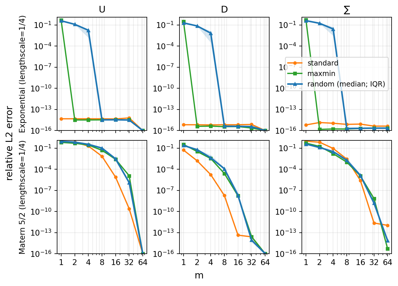
Figure 7 shows the effect of changing the ordering of the input points, then constructing neighbourhood sets using the nearest neighbours available in that ordering for 2 kernels. A consistent result is that other orderings require almost twice as many neighbours to achieve the same reconstruction error as the standard ordering. Unfortunately, order matters.

m_values = [1, 2, 4, 8, 16, 32, 64]
ms = np.array(m_values, dtype=float)
y_floor = 1e-16

# Orderings computed earlier in the notebook (see fig-ud-ordering-effects).
assert x.shape == (64, 1)
assert x_maxmin.shape == (64, 1)
assert isinstance(x_permuted, list) and len(x_permuted) == 10
assert all(xp.shape == (64, 1) for xp in x_permuted)


def nearest_neighbourhood_sets(x_order: np.ndarray, m: int) -> dict[int, list[int]]:
    # For each i, pick the min(m, i) nearest points among {0, ..., i-1}
    # under this ordering, using distance in x-space.
    n = x_order.shape[0]
    x_flat = x_order[:, 0] if x_order.ndim == 2 else x_order

    neighbourhood_sets: dict[int, list[int]] = {0: []}
    for i in range(1, n):
        prev = np.arange(i)
        k = min(m, i)
        if k == i:
            idx = prev
        else:
            dists = np.abs(x_flat[i] - x_flat[prev])
            idx = prev[np.argsort(dists)[:k]]
        neighbourhood_sets[i] = np.sort(idx).tolist()

    return neighbourhood_sets


# Neighbourhood sets depend on BOTH the ordering AND m.
nh_std_by_m = {m: nearest_neighbourhood_sets(x, m) for m in m_values}
nh_maxmin_by_m = {m: nearest_neighbourhood_sets(x_maxmin, m) for m in m_values}
nh_rand_by_m_list = [{m: nearest_neighbourhood_sets(xr, m) for m in m_values} for xr in x_permuted]


def vecchia_errors_vs_m(
    kernel: Matern, x_order: np.ndarray, nh_by_m: dict[int, dict[int, list[int]]]
) -> dict[str, np.ndarray]:
    Sigma = kernel(x_order, x_order)
    U_exact, D_exact = get_U_and_D_exact(Sigma)

    err_U = []
    err_D = []
    err_cov = []

    for m in m_values:
        U_m, D_m = get_U_and_D_vecchia(Sigma, nh_by_m[m])
        Sigma_m = reconstruct_Sigma_from_U_D(U_m, D_m)

        err_U.append(rel_l2_error(U_exact, U_m))
        err_D.append(rel_l2_error(D_exact, D_m))
        err_cov.append(rel_l2_error(Sigma, Sigma_m))

    return {
        "U": np.maximum(np.array(err_U, dtype=float), y_floor),
        "D": np.maximum(np.array(err_D, dtype=float), y_floor),
        "cov": np.maximum(np.array(err_cov, dtype=float), y_floor),
    }


kernel_keys = [(0.5, 4), (2.5, 4)]
kernel_names = [str(results[k]["name"]) for k in kernel_keys]

errors_by_kernel: list[dict[str, object]] = []
for k in kernel_keys:
    kernel, _name = params_to_kernel[k]

    std = vecchia_errors_vs_m(kernel, x, nh_std_by_m)
    mm = vecchia_errors_vs_m(kernel, x_maxmin, nh_maxmin_by_m)

    rand_samples_U = []
    rand_samples_D = []
    rand_samples_cov = []
    for x_rand, nh_rand_by_m in zip(x_permuted, nh_rand_by_m_list):
        e = vecchia_errors_vs_m(kernel, x_rand, nh_rand_by_m)
        rand_samples_U.append(e["U"])
        rand_samples_D.append(e["D"])
        rand_samples_cov.append(e["cov"])

    rand_samples_U = np.array(rand_samples_U, dtype=float)  # (10, |m|)
    rand_samples_D = np.array(rand_samples_D, dtype=float)
    rand_samples_cov = np.array(rand_samples_cov, dtype=float)

    q_U = np.quantile(rand_samples_U, [0.25, 0.5, 0.75], axis=0, method="linear")
    q_D = np.quantile(rand_samples_D, [0.25, 0.5, 0.75], axis=0, method="linear")
    q_cov = np.quantile(rand_samples_cov, [0.25, 0.5, 0.75], axis=0, method="linear")

    errors_by_kernel.append(
        {
            "standard": std,
            "maxmin": mm,
            "random_q": {"U": q_U, "D": q_D, "cov": q_cov},  # rows: q1, q2, q3
        }
    )


fig, axes = plt.subplots(
    2,
    3,
    constrained_layout=True,
    sharex=True,
    sharey="col",
)

col_keys = ["U", "D", "cov"]
col_titles = ["U", "D", "∑"]

colors = {"standard": "tab:orange", "maxmin": "tab:green", "random": "tab:blue"}

for r in range(2):
    for c, (ckey, ctitle) in enumerate(zip(col_keys, col_titles)):
        ax = axes[r, c]

        std = errors_by_kernel[r]["standard"][ckey]
        mm = errors_by_kernel[r]["maxmin"][ckey]
        q = errors_by_kernel[r]["random_q"][ckey]
        q1, q2, q3 = q[0], q[1], q[2]

        ax.plot(ms, std, marker="o", markersize=3.5, linewidth=1.6, color=colors["standard"], label="standard")
        ax.plot(ms, mm, marker="s", markersize=3.5, linewidth=1.6, color=colors["maxmin"], label="maxmin")
        ax.fill_between(ms, q1, q3, color=colors["random"], alpha=0.18, linewidth=0)
        ax.plot(ms, q2, marker="^", markersize=3.7, linewidth=2.0, color=colors["random"], label="random (median; IQR)")

        ax.set_xscale("log")
        ax.set_yscale("log")
        ax.grid(alpha=0.25, which="both")
        ax.set_ylim(bottom=y_floor, top=1.3)

        if r == 0:
            ax.set_title(ctitle)
        if c == 0:
            ax.set_ylabel(kernel_names[r])


for ax in axes[-1, :]:
    ax.set_xticks(m_values)
    ax.set_xticklabels([str(m) for m in m_values])

fig.supylabel("relative L2 error")
fig.supxlabel("m")

axes[0, 2].legend(fontsize=9, loc="best")

plt.show()
plt.close(fig)

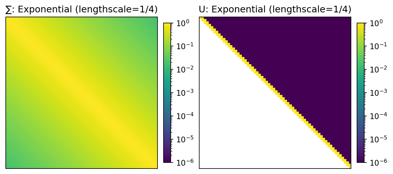
Figure 7: Relative L2 reconstruction error vs neighbourhood size m under different orderings (standard, maxmin, random). Random ordering shows median with interquartile range shading over 10 random orderings.

3.5 Summary of Section 3

The Vecchia approximation essentially uses the same factorization introduced in Section 2.1 but replaces the index set “:i” with a smaller index set N(i) \subseteq \{1, \ldots, i-1\} in the GP posterior equations, leading to a sparse matrix.

Reconstructions generally look good, although weird artifacts appear for certain kernels (e.g. RBF) or for very tiny numbers of neighbours. Ordering of the input points matters (unfortunately).

4 Vecchia on GPs (high-level overview)

Finally we will extend the Vecchia approximation to full GP models. There are essentially three issues:

1. Inference on arbitrary points
2. Posterior inference
3. Noisy observations

CautionLess detailed section

This topic is quite large and this post is already getting quite long, so this will be much less detailed than previous sections.

4.1 Inference on arbitrary points

This essentially requires defining a neighbourhood set for arbitrary input points. What makes this a bit tricky is that the neighbourhood set can only contain previous points (which implies an ordering and the presence of previous points). As far as I can tell, the way this is handled is to create a consistent rule to define the neighbourhood sets (e.g. nearest neighbours using Euclidean distance), internally track a set of points for inference and an ordering of those points, and create new neighbourhood sets dynamically as needed. Unfortunately, this introduces a kind of “history” into the model that GPs normally lack (the covariance depends explicitly on the previous points).

4.2 Posterior inference

So far we have only applied the Vecchia approximation to GP priors (effectively a multivariate Gaussian). I know of two ways to extend this to GP posteriors.

The first way (and most common in the literature) is to simply run the sequential sampling procedure as described in Section 3.3, skipping sampling of variables y_i that we are conditioning on, and substituting the observed values for those variables when sampling y_j which depend on observed y_i. You can run through the linear algebra in a similar way as before to create an explicit sparse factorization of the posterior (although I won’t do that here). This is essentially doing exact posterior inference in the approximate model, with one important caveat: it is only exact if the observed variables come before all unobserved variables in the ordering. Substituting an observed value only influences variables sampled later; any variable sampled before an observation is completely unaffected by it, whereas exact conditioning would propagate information “backwards” too. In practice this is handled by simply placing the observed points first in the ordering.

The second way is to apply the Vecchia approximation to the exact posterior covariance matrix on the evaluation set. You run the steps of the approximation as before, but any time you need a submatrix of the covariance matrix you subtract off the normal posterior adjustment term in exact GP inference.

Which one is better? Ultimately it depends on the application and number of training vs test points. For large number of training points, the first approach will be more scalable. For a small number of training points, the second approach will (probably) be more accurate.

4.3 Noisy observations

This is the trickiest case, and the bulk of Katzfuss and Guinness (2021) is effectively devoted to this topic. This is because, for noisy observations, each input point x is associated with two random variables: the latent GP function f(x) and the noisy observation y. These random variables are jointly Gaussian, and exact (uncorrelated) Gaussian noise means y is conditionally independent of all other variables given f(x).

Normally in a GP we only track the distribution of f explicitly, and calculate distributions of y as needed. However, if here we want to use the first method of posterior inference (described above), we not only need to include y in the sampling procedure, but conditioning on y will only apply to a subset of the variables. If, for example, our sampling procedure is to sample f sequentially and then sample y in terms of f (which is the most natural way to sample from the GP prior), then conditioning on y won’t actually affect any f values. On the other hand, if we sample y first and then sample f in terms of y, f might end up being biased towards y rather than f values from nearby points.

They survey a large number of different strategies to handle this conditioning, which admittedly I didn’t understand in detail.

5 Conclusions

Vecchia is a rather unique GP approximation that constructs a sparse factorization of the precision matrix of a GP but limits the non-zero entries of the factorization to be a predetermined subset of the previous points. It is effectively a kind of local approximation, and seems most accurate when each point has only a small number of conditional dependencies in the exact GP, which depends on the kernel function and its effective lengthscale.

Even though the 1D examples in the post don’t show systematic under- or over-correlation, it is still my intuition that Vecchia will tend to under-correlate points rather than over-correlate them, as low-rank methods tend to do. The approximation makes most sense when the data looks like clusters of independent points, with dependencies within each cluster. Low-rank methods are intrinsically incapable of modelling arbitrary numbers of distinct clusters, whereas Vecchia is intrinsically incapable of modelling large dependencies within a cluster.

I can see why Vecchia is useful in geospatial applications, where correlations are strong for points close in space or time, but weak between distant points. However, I suspect it is also good for other applications. The application I had in mind when looking into Vecchia was modelling molecular properties on massive datasets of molecules, which contain too many clusters to be effectively modelled by low-rank methods. I’m still trying to understand the pathologies of applying Vecchia to this kind of data.

If you are working in this field, I hope you found this helpful! I’ll end with some miscellaneous notes that didn’t fit into the main text.

NotePractical implementation of Vecchia

Here are some tips:

1. Numerical linear algebra errors can be common, and especially when calculating D. Look out for small values in D- it can ruin the approximation.
2. Although Vecchia is usually presented with a sequential construction, it’s actually a lot faster to calculate the rows in batches. Most steps involve constructing and inverting small m\times m sub-matrices of the kernel matrix, and this benefits from vectorization (especially on a GPU). I got at least a factor of 2 speedup by doing this.
3. A library like faiss to calculate approximate nearest neighbours quickly is essential; otherwise the cost of constructing the neighbourhood sets will dominate the computation.

NoteRelationship to the Cholesky factorization

The exact factorization from Section 2.1 and the Cholesky decomposition are both triangular factorizations of positive definite matrices, and this is no coincidence: they are the same object in disguise. Let \mathrm{chol}(\cdot) denote the (lower triangular) Cholesky factor.

Inverting \Sigma^{-1} = UD^{-1}U^T yields

\Sigma = U^{-T} D U^{-1} \ .

Since U^{-T} is unit lower triangular and D is a positive diagonal matrix, this is exactly the LDL^T factorization of \Sigma, which is unique, so

\mathrm{chol}(\Sigma) = U^{-T}D^{1/2} , \qquad \left(UD^{-1/2}\right)^T = \mathrm{chol}(\Sigma)^{-1} \ .

In other words, the exact factor UD^{-1/2} is the inverse transpose of the Cholesky factor of the covariance matrix. In hindsight this shouldn’t be surprising: sequentially conditioning each variable on the previous ones is precisely what the Cholesky algorithm computes. A nice corollary is that the ith diagonal entry of \mathrm{chol}(\Sigma) is the conditional standard deviation \sigma_i from Equation 1.

NoteGuide to the code in this notebook

When writing the code to produce the plots in this post, I tried to stick with simple implementations, even if they aren’t the most efficient or numerically stable.

There are also some terminology / notation changes in the code that don’t match the text in the post.

• Indexing is always done from 0, not 1 (following standard python slice semantics)
• The term “Vecchia factor” is used to refer to the (U, D) tuple (implicitly it is UD^{-1/2})

References

Katzfuss, Matthias, and Joseph Guinness. 2021. “A General Framework for Vecchia Approximations of Gaussian Processes.” Statistical Science 36 (1): pp. 124–141. https://www.jstor.org/stable/26997951.

Zhang, Lu. 2018. Nearest Neighbor Gaussian Processes (NNGP) Based Models in Stan. Https://mc-stan.org/learn-stan/case-studies/nngp.html.

Footnotes

1. Of course, these days “myself” means with heavy LLM assistance.

2. See this post for details on LLM-alpha.

3. This is arguably a feature: a sparse covariance forces independence between points, which might not be warranted.

4. Valid because with this substitution \mathrm{Cov}[\mathbf{\epsilon}] = A^T \Sigma A = A^T \left(A A^T\right)^{-1} A = I as required (using \Sigma^{-1} = A A^T). Note that the transpose matters: substituting \Sigma^{-1/2} = A instead would give \mathrm{Cov}[\mathbf{\epsilon}] = A \Sigma A^T \neq I in general. Unlike scalar square roots, the two factors in AA^T are not interchangeable.

5. If you don’t follow, go through Equation 1 for i=2, 3, ... and match it to the matrix row by row (I bet an LLM could explain in great detail).

6. I’ve added a small value of 1e-6 to all entries to avoid zeros in the logs. The actual values are likely much smaller.

7. Entries of U are generally not exactly zero, and even when they are in exact arithmetic (e.g. for the exponential kernel, whose Markov property makes all entries beyond the first off-diagonal exactly zero), floating point computation produces tiny non-zero values instead. Also, all these matrices contain values of \approx 1 in each row (near the diagonal), so entries with absolute value less than 10^{-4} will not significantly affect matrix operations and could practically be replaced by zero. This, plus numerical linear algebra being inexact is why I chose this slightly larger cutoff.

8. I think I recall reading that it is optimal in terms of KL between the true and approximate distributions, but I’m not sure, and won’t touch this subject in this post.

9. As far as I can tell this is another artifact of evaluation on a grid, and I won’t explore this in more detail.